Matlab Tutorial - Discrete Fourier Transform (DFT)

---

---

"FFT algorithms are so commonly employed to compute DFTs that the term 'FFT' is often used to mean 'DFT' in colloquial settings. Formally, there is a clear distinction: 'DFT' refers to a mathematical transformation or function, regardless of how it is computed, whereas 'FFT' refers to a specific family of algorithms for computing DFTs." - Discrete Fourier transform - http://www.princeton.edu/

The Fourier Transform of the original signal is:

$$X(j \omega ) = \int_{-\infty}^\infty x(t)e^{-j\omega t} dt$$

We take $N$ samples from $x(t)$, and those samples can be denoted as $x[0]$, $x[1]$,...,$x[n]$,...,$x[N-1]$.

Since we could think each sample $x[n]$ as an impulse which has an area of $x[n]$:

$$X(j \omega ) = \int_0^{(N-1)T} x(t)e^{-j\omega t}dt$$ $$= x[0]e^{-j0} + x[1]e^{-j\omega T} + ... + x[n]e^{-j\omega nT} + ... + x[N-1]e^{-j\omega (N-1)T}$$

So, $X(j \omega )$ becomes

$$X(j \omega ) = \sum\limits_{n=0}^{N-1}x[n]e^{-j\omega nT}$$

Since there are only a finite number of input data, the DFT treats the data as if it were period, and evaluates the equation for the fundamental frequency:

$$\omega = 0,\frac{2\pi}{NT},\frac{2\pi}{NT} \times 2, ..., \frac{2\pi}{NT} \times n,..., \frac{2\pi}{NT} \times (N-1)$$

Therefore, the Discrete Fourier Transform of the sequence $x[n]$ can be defined as:

$$X[k] = \sum\limits_{n=0}^{N-1}x[n]e^{-j2\pi kn/N} (k = 0: N-1)$$

The equation can be written in matrix form:

$$\begin{bmatrix} X[0] \\ X[1] \\ X[2] \\ . \\ . \\ . \\ X[N-1] \end{bmatrix} = \begin{bmatrix} 1 & 1 & 1 & 1 & ... & 1 \\ 1 & W & W^2 & W^3 & ... & W^{N-1} \\ 1 & W^2 & W^4 & W^6 & ... & W^{2(N-1)} \\ 1 & W^3 & W^6 & W^9 & ... & W^{3(N-1)} \\ . & . & . & . & . & . \\ . & . & . & . & . & . \\ . & . & . & . & . & . \\ 1 & W^{N-1} & W^{2(N-1)} & W^{3(N-1)} & ... & W^{(N-1)(N-1)} \\ \end{bmatrix} \begin{bmatrix} x[0] \\ x[1] \\ x[2] \\ . \\ . \\ . \\ x[N-1] \end{bmatrix} $$

where $W = e^{-j2\pi / N}$ and $W = W^{2N} = 1 $.

Quite a few people use $W_N$ for $W$.

So, our final DFT equation can be defined like this:

$$X[k] = \sum\limits_{n=0}^{N-1}x[n]W^{kn}_N ~~ (k = 0: N-1)$$

The inverse of it:

$$x[n] = \frac{1}{N} \sum\limits_{n=0}^{N-1}X[k]W^{-kn}_N ~~ (k = 0: N-1)$$

Here is a simple example without using the built in function.

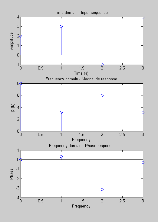
$$x[n] = [2 ~ 3 ~ -1 ~ 4]$$ $$X[k] = \sum\limits_{n=0}^3x[n]e^{-j\pi n k /2} = \sum\limits_{n=0}^3x[n](-j)^{n k}$$ $$X[0] = 2 + 3 + (=1) + 4 =8 $$ $$X[1] = 2 + (-3j) + 1 + 4j = 3 + j$$ $$X[2] = 2 + (-3) + (-1) -4 = -6 $$ $$X[3] = 2 + (3j) + 1 -4j = 3 -j $$

The Matlab code looks like this:

x = [2 3 -1 4];
N = length(x);
X = zeros(4,1)
for k = 0:N-1
    for n = 0:N-1
        X(k+1) = X(k+1) + x(n+1)*exp(-j*pi/2*n*k)
    end
end

t = 0:N-1
subplot(311)
stem(t,x);
xlabel('Time (s)');
ylabel('Amplitude');
title('Time domain - Input sequence')

subplot(312)
stem(t,X)
xlabel('Frequency');
ylabel('|X(k)|');
title('Frequency domain - Magnitude response')

subplot(313)
stem(t,angle(X))
xlabel('Frequency');
ylabel('Phase');
title('Frequency domain - Phase response')

X         % to check |X(k)|
angle(X)  % to check phase

If we run the script, we get:

X =
   8.0000 + 0.0000i
   3.0000 + 1.0000i
  -6.0000 - 0.0000i
   3.0000 - 1.0000i

ans =

         0
    0.3218
   -3.1416
   -0.3218

The response $X[k]$ is what we expected and it gives exactly the same as we calculated. The plots are:

In this section, instead of doing it manually, we do it using fft() provided by Matlab. Here is the code:

N=4;
x=[2 3 -1 4];

t=0:N-1;
subplot(311)
stem(t,x);
xlabel('Time (s)');
ylabel('Amplitude');
title('Input sequence')

subplot(312); 
stem(0:N-1,abs(fft(x)));  
xlabel('Frequency');
ylabel('|X(k)|');
title('Magnitude Response'); 

subplot(313); 
stem(0:N-1,angle(fft(x)));
xlabel('Frequency');
ylabel('Phase');
title('Phase Response'); 

We'll get the identical results as in the previous section.