BogoToBogo
  • Home
  • About
  • Big Data
  • Machine Learning
  • AngularJS
  • Python
  • C++
  • go
  • DevOps
  • Kubernetes
  • Algorithms
  • More...
    • Qt 5
    • Linux
    • FFmpeg
    • Matlab
    • Django 1.8
    • Ruby On Rails
    • HTML5 & CSS

Signal Processing with NumPy arrays in iPython

OpenCV_Logo.png


Bookmark and Share


bogotobogo.com site search:

iPython

IPython currently provides the following features (wiki-iPython):

  1. Powerful interactive shells (terminal and Qt-based).
  2. A browser-based notebook with support for code, text, mathematical expressions, inline plots and other rich media.
  3. Support for interactive data visualization and use of GUI toolkits.
  4. Flexible, embeddable interpreters to load into ones own projects.
  5. Easy to use, high performance tools for parallel computing.


bogotobogo.com site search:


Note

We're not going deep into the signal processing but mainly focused on iPython and plot with very basic array operations.


Basic Signals - boxcar

We'll make a simple boxcar with np.zeros() and np.ones().

We start with a simple command to get python environment using ipython --pylab:

$ ipython --pylab
Python 2.7.5+ (default, Feb 27 2014, 19:37:08) 
Type "copyright", "credits" or "license" for more information.

IPython 0.13.2 -- An enhanced Interactive Python.
?         -> Introduction and overview of IPython's features.
%quickref -> Quick reference.
help      -> Python's own help system.
object?   -> Details about 'object', use 'object?' for extra details.

Welcome to pylab, a matplotlib-based Python environment [backend: TkAgg].
For more information, type 'help(pylab)'.

In [1]: 

Let's play with arrays first:

In [1]: zeros
Out[1]: 

In [2]: zeros(100)
Out[2]: 
array([ 0.,  0.,  0.,  0.,  0.,  0.,  0.,  0.,  0.,  0.,  0.,  0.,  0.,
        0.,  0.,  0.,  0.,  0.,  0.,  0.,  0.,  0.,  0.,  0.,  0.,  0.,
        0.,  0.,  0.,  0.,  0.,  0.,  0.,  0.,  0.,  0.,  0.,  0.,  0.,
        0.,  0.,  0.,  0.,  0.,  0.,  0.,  0.,  0.,  0.,  0.,  0.,  0.,
        0.,  0.,  0.,  0.,  0.,  0.,  0.,  0.,  0.,  0.,  0.,  0.,  0.,
        0.,  0.,  0.,  0.,  0.,  0.,  0.,  0.,  0.,  0.,  0.,  0.,  0.,
        0.,  0.,  0.,  0.,  0.,  0.,  0.,  0.,  0.,  0.,  0.,  0.,  0.,
        0.,  0.,  0.,  0.,  0.,  0.,  0.,  0.,  0.])
In [3]: ones(10)
Out[3]: array([ 1.,  1.,  1.,  1.,  1.,  1.,  1.,  1.,  1.,  1.])

Now, we want to concatenate these and make a boxcar:

Also, we we know more about the command, we can add '?' after the command. Then, it will show details about the command as well as some usage samples:

In [4]: concatenate?

The following information will be displayed in another window (I mean if we can close the help window (by typing 'q'), our command shell will reappear:

Type:       builtin_function_or_method
String Form:<built-in function concatenate>
Docstring:
concatenate((a1, a2, ...), axis=0)

Join a sequence of arrays together.

Parameters
----------
a1, a2, ... : sequence of array_like
    The arrays must have the same shape, except in the dimension
    corresponding to `axis` (the first, by default).
axis : int, optional
    The axis along which the arrays will be joined.  Default is 0.

Now, concatenation:

In [5]: concatenate ( (zeros(100), ones(30), zeros(100)) )
Out[5]: 
array([ 0.,  0.,  0.,  0.,  0.,  0.,  0.,  0.,  0.,  0.,  0.,  0.,  0.,
        0.,  0.,  0.,  0.,  0.,  0.,  0.,  0.,  0.,  0.,  0.,  0.,  0.,
        0.,  0.,  0.,  0.,  0.,  0.,  0.,  0.,  0.,  0.,  0.,  0.,  0.,
        0.,  0.,  0.,  0.,  0.,  0.,  0.,  0.,  0.,  0.,  0.,  0.,  0.,
        0.,  0.,  0.,  0.,  0.,  0.,  0.,  0.,  0.,  0.,  0.,  0.,  0.,
        0.,  0.,  0.,  0.,  0.,  0.,  0.,  0.,  0.,  0.,  0.,  0.,  0.,
        0.,  0.,  0.,  0.,  0.,  0.,  0.,  0.,  0.,  0.,  0.,  0.,  0.,
        0.,  0.,  0.,  0.,  0.,  0.,  0.,  0.,  0.,  1.,  1.,  1.,  1.,
        1.,  1.,  1.,  1.,  1.,  1.,  1.,  1.,  1.,  1.,  1.,  1.,  1.,
        1.,  1.,  1.,  1.,  1.,  1.,  1.,  1.,  1.,  1.,  1.,  1.,  1.,
        0.,  0.,  0.,  0.,  0.,  0.,  0.,  0.,  0.,  0.,  0.,  0.,  0.,
        0.,  0.,  0.,  0.,  0.,  0.,  0.,  0.,  0.,  0.,  0.,  0.,  0.,
        0.,  0.,  0.,  0.,  0.,  0.,  0.,  0.,  0.,  0.,  0.,  0.,  0.,
        0.,  0.,  0.,  0.,  0.,  0.,  0.,  0.,  0.,  0.,  0.,  0.,  0.,
        0.,  0.,  0.,  0.,  0.,  0.,  0.,  0.,  0.,  0.,  0.,  0.,  0.,
        0.,  0.,  0.,  0.,  0.,  0.,  0.,  0.,  0.,  0.,  0.,  0.,  0.,
        0.,  0.,  0.,  0.,  0.,  0.,  0.,  0.,  0.,  0.,  0.,  0.,  0.,
        0.,  0.,  0.,  0.,  0.,  0.,  0.,  0.,  0.])

Actually, we want to assign the array to a variable:

In [6]: data  = concatenate ( (zeros(100), ones(30), zeros(100)) )

In [7]: plot(data)
Out[7]: [<matplotlib.lines.Line2D at 0x3024450>]

The we get the picture below:


iPython_boxcar.png

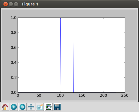
Note the values in the array is for y-values, for x-axis, the sample numbers are used: we have 100+30+100=230 samples.


Hamming filter
In [8]: hamming(40)
Out[8]: 
array([ 0.08      ,  0.08595688,  0.10367324,  0.13269023,  0.17225633,
        0.2213468 ,  0.27869022,  0.34280142,  0.41201997,  0.48455313,
        0.55852233,  0.63201182,  0.70311825,  0.77      ,  0.83092487,
        0.88431494,  0.92878744,  0.96319054,  0.98663324,  0.99850836,
        0.99850836,  0.98663324,  0.96319054,  0.92878744,  0.88431494,
        0.83092487,  0.77      ,  0.70311825,  0.63201182,  0.55852233,
        0.48455313,  0.41201997,  0.34280142,  0.27869022,  0.2213468 ,
        0.17225633,  0.13269023,  0.10367324,  0.08595688,  0.08      ])

In [9]: plot(hamming(40))
Out[9]: []

Then, we get the following picture:


iPython_Hamming.png

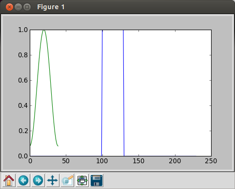
We overwrote a new to the old one because we did not close the plot window before we made a new draw.

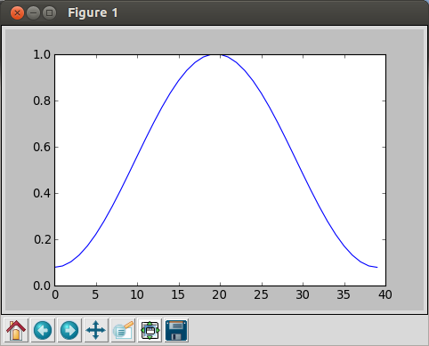
So, let's close this window, and plot the Hamming again:

In [10]: plot(hamming(40))
Out[10]: []

Now, we have a plot with only the Hamming filter:


iPython_Hamming_only.png

However, if we want to apply the filter to the other signal, we need to normalize the filter.


Normalizing the Hamming filter

We'll normalize the filter by diving it by the sum of the filter values:

In [11]: sum(hamming(40))
Out[11]: 21.139999999999997

In [12]: norm = hamming(40) / sum(hamming(40))

In [13]: plot(norm)
Out[13]: []

The we get normalized Hamming filter:


iPython_Hamming_Normalized.png

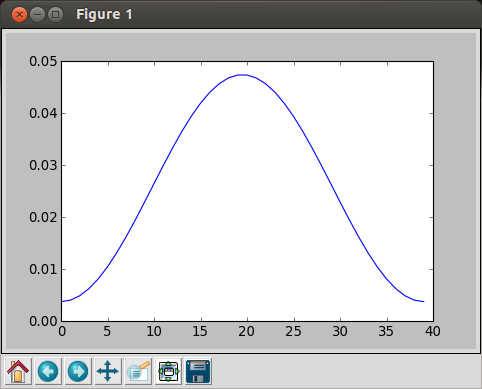
Note that the peak value is much lower than the previous Hamming filter.


Convolve

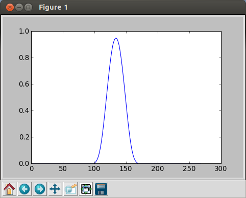
Now we do convolve the filter with the boxcar data:

In [14]: convolve(data, norm)
Out[14]: 
array([ 0.        ,  0.        ,  0.        ,  0.        ,  0.        ,
        0.        ,  0.        ,  0.        ,  0.        ,  0.        ,
        0.        ,  0.        ,  0.        ,  0.        ,  0.        ,
        0.        ,  0.        ,  0.        ,  0.        ,  0.        ,
        0.        ,  0.        ,  0.        ,  0.        ,  0.        ,
        0.        ,  0.        ,  0.        ,  0.        ,  0.        ,
        0.        ,  0.        ,  0.        ,  0.        ,  0.        ,
        0.        ,  0.        ,  0.        ,  0.        ,  0.        ,
        0.        ,  0.        ,  0.        ,  0.        ,  0.        ,
        0.        ,  0.        ,  0.        ,  0.        ,  0.        ,
        0.        ,  0.        ,  0.        ,  0.        ,  0.        ,
        0.        ,  0.        ,  0.        ,  0.        ,  0.        ,
        0.        ,  0.        ,  0.        ,  0.        ,  0.        ,
        0.        ,  0.        ,  0.        ,  0.        ,  0.        ,
        0.        ,  0.        ,  0.        ,  0.        ,  0.        ,
        0.        ,  0.        ,  0.        ,  0.        ,  0.        ,
        0.        ,  0.        ,  0.        ,  0.        ,  0.        ,
        0.        ,  0.        ,  0.        ,  0.        ,  0.        ,
        0.        ,  0.        ,  0.        ,  0.        ,  0.        ,
        0.        ,  0.        ,  0.        ,  0.        ,  0.        ,
        0.0037843 ,  0.00785037,  0.0127545 ,  0.01903124,  0.0271796 ,
        0.03765012,  0.05083319,  0.06704896,  0.08653903,  0.10946018,
        0.13588035,  0.16577684,  0.19903693,  0.23546077,  0.27476658,
        0.31659794,  0.36053301,  0.40609548,  0.45276687,  0.5       ,
        0.54723313,  0.59390452,  0.63946699,  0.68340206,  0.72523342,
        0.76453923,  0.80096307,  0.83422316,  0.86411965,  0.89053982,
        0.90967668,  0.92510066,  0.93641231,  0.94331865,  0.94564081,
        0.94331865,  0.93641231,  0.92510066,  0.90967668,  0.89053982,
        0.86411965,  0.83422316,  0.80096307,  0.76453923,  0.72523342,
        0.68340206,  0.63946699,  0.59390452,  0.54723313,  0.5       ,
        0.45276687,  0.40609548,  0.36053301,  0.31659794,  0.27476658,
        0.23546077,  0.19903693,  0.16577684,  0.13588035,  0.10946018,
        0.08653903,  0.06704896,  0.05083319,  0.03765012,  0.0271796 ,
        0.01903124,  0.0127545 ,  0.00785037,  0.0037843 ,  0.        ,
        0.        ,  0.        ,  0.        ,  0.        ,  0.        ,
        0.        ,  0.        ,  0.        ,  0.        ,  0.        ,
        0.        ,  0.        ,  0.        ,  0.        ,  0.        ,
        0.        ,  0.        ,  0.        ,  0.        ,  0.        ,
        0.        ,  0.        ,  0.        ,  0.        ,  0.        ,
        0.        ,  0.        ,  0.        ,  0.        ,  0.        ,
        0.        ,  0.        ,  0.        ,  0.        ,  0.        ,
        0.        ,  0.        ,  0.        ,  0.        ,  0.        ,
        0.        ,  0.        ,  0.        ,  0.        ,  0.        ,
        0.        ,  0.        ,  0.        ,  0.        ,  0.        ,
        0.        ,  0.        ,  0.        ,  0.        ,  0.        ,
        0.        ,  0.        ,  0.        ,  0.        ,  0.        ,
        0.        ,  0.        ,  0.        ,  0.        ,  0.        ,
        0.        ,  0.        ,  0.        ,  0.        ,  0.        ,
        0.        ,  0.        ,  0.        ,  0.        ,  0.        ,
        0.        ,  0.        ,  0.        ,  0.        ,  0.        ,
        0.        ,  0.        ,  0.        ,  0.        ,  0.        ,
        0.        ,  0.        ,  0.        ,  0.        ,  0.        ,
        0.        ,  0.        ,  0.        ,  0.        ,  0.        ,
        0.        ,  0.        ,  0.        ,  0.        ])

In [15]: 

If we plot, it looks like this:


iPython_convolve.png


Random Signal and FFT

We can also generate random signals.

In [16]: randn(20)
Out[16]: 
array([ 1.04943265, -1.10655086,  2.65115344,  0.37216869, -1.81576411,
       -0.72413097, -0.74942176, -0.38411864,  0.04484577,  0.31172929,
       -0.78896659, -0.47319888, -0.61743916, -0.77453274, -2.34677579,
       -0.61554551,  0.93594151, -1.06451913, -1.13374368,  1.16034994])

If we do FFT with 100 random numbers:

In [17]: random_data = randn(100)

In [18]: plot(fft.fft(random_data))
/usr/lib/python2.7/dist-packages/numpy/core/numeric.py:320: ComplexWarning: Casting complex values to real discards the imaginary part
  return array(a, dtype, copy=False, order=order)
Out[18]: []

In [19]: plot(random_data)
Out[19]: []

In [20]: 

iPython_FFT_Random.png

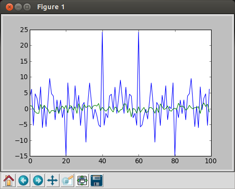
blue: FFT, green = random data


OpenCV 3 Tutorial

image & video processing


Installing on Ubuntu 13

Mat(rix) object (Image Container)

Creating Mat objects

The core : Image - load, convert, and save

Smoothing Filters A - Average, Gaussian

Smoothing Filters B - Median, Bilateral


OpenCV 3 image and video processing with Python


OpenCV 3 with Python

Image - OpenCV BGR : Matplotlib RGB

Basic image operations - pixel access

iPython - Signal Processing with NumPy

Signal Processing with NumPy I - FFT and DFT for sine, square waves, unitpulse, and random signal

Signal Processing with NumPy II - Image Fourier Transform : FFT & DFT

Inverse Fourier Transform of an Image with low pass filter: cv2.idft()

Image Histogram

Video Capture and Switching colorspaces - RGB / HSV

Adaptive Thresholding - Otsu's clustering-based image thresholding

Edge Detection - Sobel and Laplacian Kernels

Canny Edge Detection

Hough Transform - Circles

Watershed Algorithm : Marker-based Segmentation I

Watershed Algorithm : Marker-based Segmentation II

Image noise reduction : Non-local Means denoising algorithm

Image object detection : Face detection using Haar Cascade Classifiers

Image segmentation - Foreground extraction Grabcut algorithm based on graph cuts

Image Reconstruction - Inpainting (Interpolation) - Fast Marching Methods

Video : Mean shift object tracking

Machine Learning : Clustering - K-Means clustering I

Machine Learning : Clustering - K-Means clustering II

Machine Learning : Classification - k-nearest neighbors (k-NN) algorithm


Ph.D. / Golden Gate Ave, San Francisco / Seoul National Univ / Carnegie Mellon / UC Berkeley / DevOps / Deep Learning / Visualization

YouTubeMy YouTube channel

Sponsor Open Source development activities and free contents for everyone.

Thank you.

- K Hong


OpenCV 3 image and video processing with Python


OpenCV 3 with Python

Image - OpenCV BGR : Matplotlib RGB

Basic image operations - pixel access

iPython - Signal Processing with NumPy

Signal Processing with NumPy I - FFT and DFT for sine, square waves, unitpulse, and random signal

Signal Processing with NumPy II - Image Fourier Transform : FFT & DFT

Inverse Fourier Transform of an Image with low pass filter: cv2.idft()

Image Histogram

Video Capture and Switching colorspaces - RGB / HSV

Adaptive Thresholding - Otsu's clustering-based image thresholding

Edge Detection - Sobel and Laplacian Kernels

Canny Edge Detection

Hough Transform - Circles

Watershed Algorithm : Marker-based Segmentation I

Watershed Algorithm : Marker-based Segmentation II

Image noise reduction : Non-local Means denoising algorithm

Image object detection : Face detection using Haar Cascade Classifiers

Image segmentation - Foreground extraction Grabcut algorithm based on graph cuts

Image Reconstruction - Inpainting (Interpolation) - Fast Marching Methods

Video : Mean shift object tracking

Machine Learning : Clustering - K-Means clustering I

Machine Learning : Clustering - K-Means clustering II

Machine Learning : Classification - k-nearest neighbors (k-NN) algorithm

Sponsor Open Source development activities and free contents for everyone.

Thank you.

- K Hong


Python tutorial


Python Home

Introduction

Running Python Programs (os, sys, import)

Modules and IDLE (Import, Reload, exec)

Object Types - Numbers, Strings, and None

Strings - Escape Sequence, Raw String, and Slicing

Strings - Methods

Formatting Strings - expressions and method calls

Files and os.path

Traversing directories recursively

Subprocess Module

Regular Expressions with Python

Regular Expressions Cheat Sheet

Object Types - Lists

Object Types - Dictionaries and Tuples

Functions def, *args, **kargs

Functions lambda

Built-in Functions

map, filter, and reduce

Decorators

List Comprehension

Sets (union/intersection) and itertools - Jaccard coefficient and shingling to check plagiarism

Hashing (Hash tables and hashlib)

Dictionary Comprehension with zip

The yield keyword

Generator Functions and Expressions

generator.send() method

Iterators

Classes and Instances (__init__, __call__, etc.)

if__name__ == '__main__'

argparse

Exceptions

@static method vs class method

Private attributes and private methods

bits, bytes, bitstring, and constBitStream

json.dump(s) and json.load(s)

Python Object Serialization - pickle and json

Python Object Serialization - yaml and json

Priority queue and heap queue data structure

Graph data structure

Dijkstra's shortest path algorithm

Prim's spanning tree algorithm

Closure

Functional programming in Python

Remote running a local file using ssh

SQLite 3 - A. Connecting to DB, create/drop table, and insert data into a table

SQLite 3 - B. Selecting, updating and deleting data

MongoDB with PyMongo I - Installing MongoDB ...

Python HTTP Web Services - urllib, httplib2

Web scraping with Selenium for checking domain availability

REST API : Http Requests for Humans with Flask

Blog app with Tornado

Multithreading ...

Python Network Programming I - Basic Server / Client : A Basics

Python Network Programming I - Basic Server / Client : B File Transfer

Python Network Programming II - Chat Server / Client

Python Network Programming III - Echo Server using socketserver network framework

Python Network Programming IV - Asynchronous Request Handling : ThreadingMixIn and ForkingMixIn

Python Coding Questions I

Python Coding Questions II

Python Coding Questions III

Python Coding Questions IV

Python Coding Questions V

Python Coding Questions VI

Python Coding Questions VII

Python Coding Questions VIII

Python Coding Questions IX

Python Coding Questions X

Image processing with Python image library Pillow

Python and C++ with SIP

PyDev with Eclipse

Matplotlib

Redis with Python

NumPy array basics A

NumPy Matrix and Linear Algebra

Pandas with NumPy and Matplotlib

Celluar Automata

Batch gradient descent algorithm

Longest Common Substring Algorithm

Python Unit Test - TDD using unittest.TestCase class

Simple tool - Google page ranking by keywords

Google App Hello World

Google App webapp2 and WSGI

Uploading Google App Hello World

Python 2 vs Python 3

virtualenv and virtualenvwrapper

Uploading a big file to AWS S3 using boto module

Scheduled stopping and starting an AWS instance

Cloudera CDH5 - Scheduled stopping and starting services

Removing Cloud Files - Rackspace API with curl and subprocess

Checking if a process is running/hanging and stop/run a scheduled task on Windows

Apache Spark 1.3 with PySpark (Spark Python API) Shell

Apache Spark 1.2 Streaming

bottle 0.12.7 - Fast and simple WSGI-micro framework for small web-applications ...

Flask app with Apache WSGI on Ubuntu14/CentOS7 ...

Selenium WebDriver

Fabric - streamlining the use of SSH for application deployment

Ansible Quick Preview - Setting up web servers with Nginx, configure enviroments, and deploy an App

Neural Networks with backpropagation for XOR using one hidden layer

NLP - NLTK (Natural Language Toolkit) ...

RabbitMQ(Message broker server) and Celery(Task queue) ...

OpenCV3 and Matplotlib ...

Simple tool - Concatenating slides using FFmpeg ...

iPython - Signal Processing with NumPy

iPython and Jupyter - Install Jupyter, iPython Notebook, drawing with Matplotlib, and publishing it to Github

iPython and Jupyter Notebook with Embedded D3.js

Downloading YouTube videos using youtube-dl embedded with Python

Machine Learning : scikit-learn ...

Django 1.6/1.8 Web Framework ...


Contact

BogoToBogo
contactus@bogotobogo.com

Follow Bogotobogo

About Us

contactus@bogotobogo.com

YouTubeMy YouTube channel
Pacific Ave, San Francisco, CA 94115

Pacific Ave, San Francisco, CA 94115

Copyright © 2024, bogotobogo
Design: Web Master