Matlab Tutorial : Vectors and Matrices

MATLAB is based on matrix and vector algebra. So, even scalars are treated as $1 \times 1$ matrices.

We have two ways to define vectors:

1. Arbitrary element (not equally spaced elements):
   

   >> v = [1 2 5];
   

   This creates a $1 \times 3$ vector with elements 1, 2 and 5. Note that commas could have been used in place of spaces to separate the elements, like this:

    
   >> v = [1, 2, 5];
   

   Keep in mind that we the index of the first element is 1 not 0:

   >> v(0)
   Subscript indices must either be real positive integers or logicals.
   >> v(1)
   ans =
        1
   

   If we want to add more elements:

   >> v(4) = 10;
   

   The yields the vector $v = [1,2,5,10]$.

   We can also use previously defined vector:

   >> >> w = [11 12];
   >> x = [v,w]
   

   Now, $x = [1, 2, 5, 10, 11, 12,]$

2. Equally spaced elements :

   >> t = 0 : .5 : 3
   

   This yields $t=[0 ~ 0.5000 ~ 1.0000 ~ 1.5000 ~ 2.0000 ~ 2.5000 ~ 3.0000]$ which is a $1 \times 7$ vector. If we give only two numbers, then the increment is set to a default of 1:

   >> t = 0:3;
   

   This will creates a $1 \times 4$ vector with the elements 0, 1, 2, 3.

One more, adding vectors:

>> u = [1 2 3];
>> v = 4 5 6];
>> w = u + v
w =
     5     7     9

We can create column vectors. In Matlab, we use semicolon(';') to separate columns:

>> RowVector = [1 2 3]   % 1 x 3 matrix
RowVector =
     1     2     3

>> ColVector = [1;2;3]   % 3 x 1 matrix
ColVector =
     1
     2
     3

>> M = [1 2 3; 4 5 6]    % 2 x 3 matrix

M =

     1     2     3
     4     5     6

Matrices are defined by entering the elements row by row:

>> M = [1 2 3; 4 5 6]
M =
     1     2     3
     4     5     6

There are a number of special matrices:

If we want to assign a new value for a particular element of a matrix (2nd row, 3rd column):

M(2,3) = 99;

We can access an element of a matrix in two ways:

1. M(row, column)
2. M(n-th_element)

>> M = [10 20 30 40 50; 60 70 80 90 100];
>> M
M =
    10    20    30    40    50
    60    70    80    90   100
 
>> M(2,4) % 2nd row 4th column
ans =
    90

>> M(8)  % 8th element 10, 60, 20, 70, 30, 80, 40, 90...
ans =
    90

Also, we can access several elements at once:

>> M(1:2, 3:4)  % row 1 2, column 3 4
ans =
    30    40
    80    90
>> M(5:8)   % from 5th to 8th elements
ans =
    30    80    40    90

If we use dot('.') on an operation, it means do it for all elements. The example does ^3 for all the elements of a matrix:

>> M = [1 2 3; 4 5 6; 7 8 9];
>> M
M =
     1     2     3
     4     5     6
     7     8     9

>> M.^3
ans =
     1     8    27
    64   125   216
   343   512   729

We can get inverse of each element:

>> 1./M
ans =
    1.0000    0.5000    0.3333
    0.2500    0.2000    0.1667
    0.1429    0.1250    0.1111

We get inverse of a matrix using inv():

>> M = [1 2; 3 4]
M =
     1     2
     3     4

>> inv(M)
ans =
   -2.0000    1.0000
    1.5000   -0.5000

We get transpose of a matrix using a single quote("'"):

>> M = [1 2 3; 4 5 6; 7 8 9]
M =
     1     2     3
     4     5     6
     7     8     9

>> M'
ans =
     1     4     7
     2     5     8
     3     6     9

flipud(): flip up/down:

>> M = [1 2 3; 4 5 6; 7 8 9]
M =
     1     2     3
     4     5     6
     7     8     9

>> flipud(M)
ans =
     7     8     9
     4     5     6
     1     2     3

fliplr(): flip left/right:

>> M
M =
     1     2     3
     4     5     6
     7     8     9

>> fliplr(M)
ans =

     3     2     1
     6     5     4
     9     8     7

We can do rotate elements, for instance, 90 degree counter-clock wise:

>> M

M =

     1     2     3
     4     5     6
     7     8     9

>> rot90(M)

ans =

     3     6     9
     2     5     8
     1     4     7

We can make a change to the number of rows and columns as far as we keep the total number of elements:

>> M = [1 2 3 4; 5 6 7 8; 9 10 11 12]
M =
     1     2     3     4
     5     6     7     8
     9    10    11    12

>> reshape(M, 2, 6)  % Convert M to 2x6 matrix
ans =
     1     9     6     3    11     8
     5     2    10     7     4    12

Functions are applied element by element:

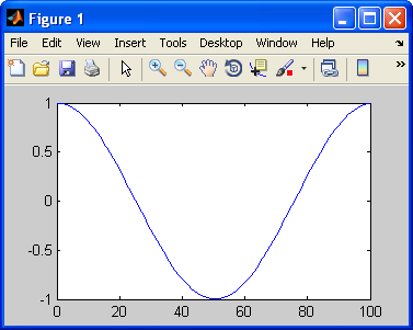
>> t = 0:100;
>> f = cos(2*pi*t/length(t))
>> plot(t,f)

$f = cos(2 \pi t/length(t))$ creates a vector $f$ with elements equal to $2 \pi t/length(t)$ for $t = 0, 1, 2, ..., 100$.