Artificial Neural Network (ANN) 2 - Forward Propagation

bogotobogo.com site search:

Forward Propagation

Continued from Artificial Neural Network (ANN) 1 - Introduction.
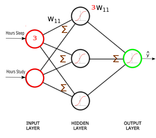
Neural-Network-3-Layers-Red-Green-Hours-Sleep-Study-Sigmoid-and-Sigma-with-3w11.png

Our network has 2 inputs, 3 hidden units, and 1 output.

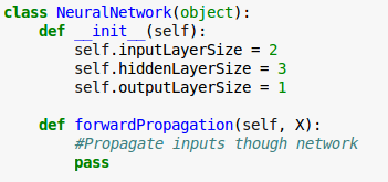
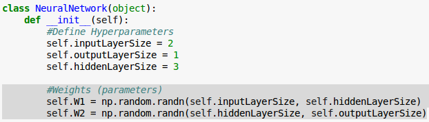
This time we'll build our network as a python class.

The init() method of the class will take care of instantiating constants and variables.

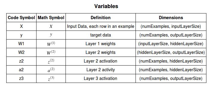
$$ \begin{align}z^{(2)} = XW^{(1)} \tag 1\\ a^{(2)} = f \left( z^{(2)} \right)& \tag 2\\ z^{(3)} = a^{(2)} W^{(2)} \tag 3\\ \hat y = f \left( z^{(3)} \right) \tag 4 \end{align} $$

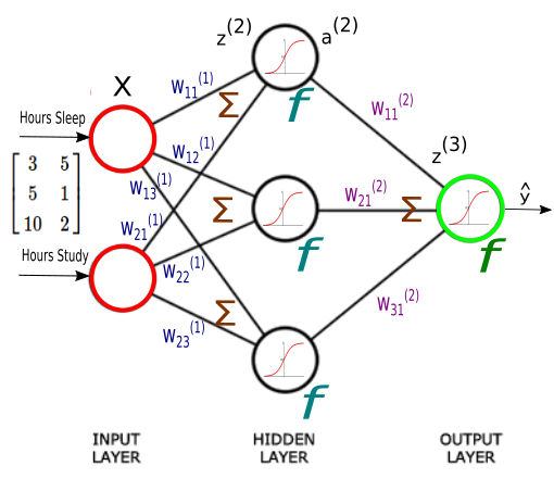
Each input value in matrix $X$ should be multiplied by a corresponding weight and then added together with all the other results for each neuron.

$z^{(2)}$ is the activity of our second layer and it can be calculated as the following:

$$ z^{(2)} = XW^{(1)} \tag 1 $$ $$ = \begin{bmatrix} 3 & 5 \\ 5 & 1 \\ 10 & 2 \end{bmatrix} \begin{bmatrix} W_{11}^{(1)} & W_{12}^{(1)} & W_{13}^{(1)}\\ W_{21}^{(1)} & W_{22}^{(1)} & W_{23}^{(1)} \end{bmatrix} $$ $$ = \begin{bmatrix} 3 W_{11}^{(1)} + 5 W_{21}^{(1)} & 3 W_{12}^{(1)} + 5 W_{22}^{(1)} & 3 W_{13}^{(1)} + 5 W_{23}^{(1)} \\ 5 W_{11}^{(1)} + W_{21}^{(1)} & 5 W_{12}^{(1)} + W_{22}^{(1)} & 5 W_{13}^{(1)} + W_{23}^{(1)} \\ 10 W_{11}^{(1)} + 2 W_{21}^{(1)} & 10 W_{12}^{(1)} + 2 W_{22}^{(1)} & 10 W_{13}^{(1)} + 2 W_{23}^{(1)} \end{bmatrix} $$

Note that each entry in $z$ is a sum of weighted inputs to each hidden neuron. $z$ is $3 \times 3$ matrix, one row for each sample, and one column for each hidden unit.

Activation function - sigmoid

Now that we have the activities for our second layer, $ z^{(2)} = XW^{(1)} $, we need to apply the activation function.

We'll independently apply the sigmoid function to each entry in matrix $z$:

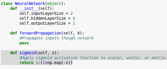
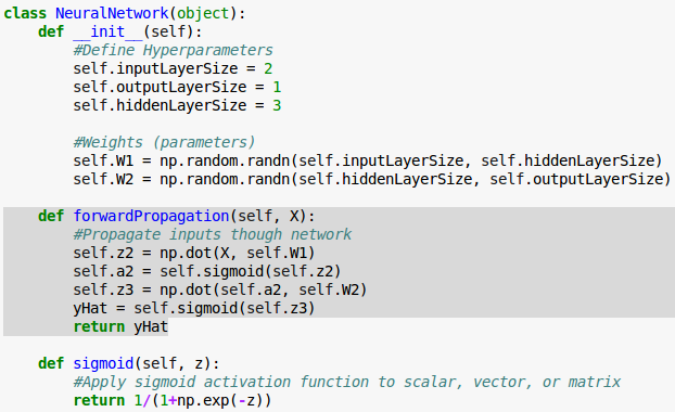
By using numpy we'll apply the activation function element-wise, and return a result of the same dimension as it was given:

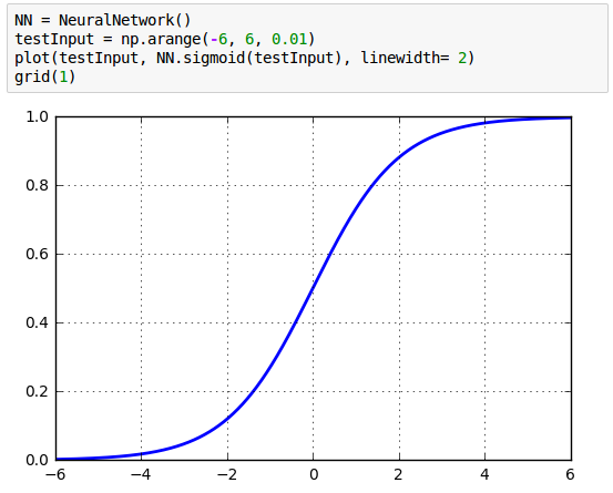
Let's see how the sigmoid() takes an input and how returns the result:

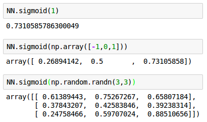
The following calls for the sigmoid() with args : a number (scalar), 1-D (vector), and 2-D arrays (matrix).

Weight-matrices : $W^{(1)}$ and $W^{(2)}$

We initialize our weight matrices ($W^{(1)}$ and $W^{(2)}$) in our __init__() method with random numbers.

Implementing forward propagation

We now have our second formula for forward propagation, using our activation function($f$), we can write that our second layer activity: $a^{(2)} = f \left( z^{(2)} \right)$. The $a^{(2)}$ will be a matrix of the same size ($3 \times 3$):

$$ a^{(2)} = f(z^{(2)}) \tag 2 $$

To finish forward propagation we want to propagate $a^{(2)}$ all the way to the output, $\hat y$.

All we have to do now is multiply $a^{(2)}$ by our second layer weights $W^{(2)}$ and apply one more activation function. The $W^{(2)}$ will be of size $3 \times 1$, one weight for each synapse:

$$ z^{(3)} = a^{(2)} W^{(2)} \tag 3 $$

Multiplying $a^{(2)}$, a ($3 \times 3$ matrix), by $W^{(2)}$, a ($3 \times 1$ matrix) results in a $3 \times 1$ matrix $z^{(3)}$, the activity of our 3rd layer. The $z^{(3)}$ has three activity values, one for each sample.

Then, we'll apply our activation function to $z^{(3)}$ yielding our estimate of test score, $\hat y$:

$$ \hat y = f \left( z^{(3)} \right) \tag 4 $$

Now we are ready to implement forward propagation in our forwardPropagation() method, using numpy's built in dot method for matrix multiplication:

Getting estimate of test score

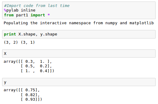
Now we have a class capable of estimating our test score given how many hours we sleep and how many hours we study. We pass in our input data ($X$) and get real outputs ($\hat y$).

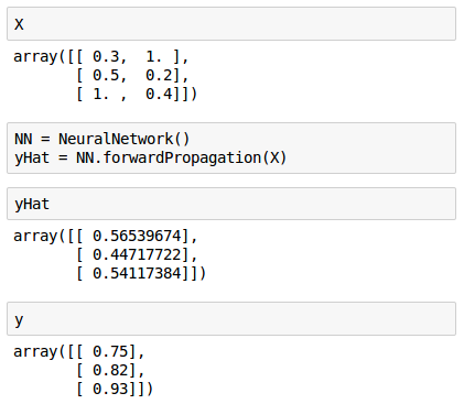
Note that our estimates ($\hat y$) looks quite terrible when compared with our target ($y$). That's because we have not yet trained our network, that's what we'll work on next article.

Next:

3. Gradient Descent