scikit-learn : Support Vector Machines (SVM) II

---

---

Continued from scikit-learn : Support Vector Machines (SVM).

Though we implemented our own classification algorithms, actually, SVM also can do the same.

First, we need to import:

from sklearn.linear_model import SGDClassifier

Then, call the following methods:

1. stochastic gradient descent version of the perceptron : Single Layer Neural Network : Adaptive Linear Neuron using linear (identity) activation function with stochastic gradient descent (SGD)

   ppn = SGDClassifier(loss='perceptron')
   

2. logistic regression : Logistic Regression

   lr = SGDClassifier(loss='log')
   

3. support vector machine with default parameters : scikit-learn : Support Vector Machines (SVM)

   svm = SGDClassifier(loss='hinge')
   

One of the reasons why SVMs enjoy popularity in machine learning is that they can be easily kernelized to solve nonlinear classification problems.

Before we discuss the main concept behind kernel SVM, we want to define and create a sample dataset to see how such a nonlinear classification problem looks like.

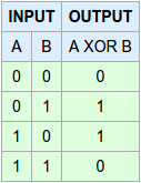
Using the following code, we will create a simple dataset that has the form of an XOR gate using the logical_xor function from NumPy:

import numpy as np
np.random.seed(0)
X_xor = np.random.randn(200, 2)
y_xor = np.logical_xor(X_xor[:, 0] > 0, X_xor[:, 1] > 0)
y_xor = np.where(y_xor, 1, -1)
plt.scatter(X_xor[y_xor==1, 0], X_xor[y_xor==1, 1], c='b', marker='x', label='1')
plt.scatter(X_xor[y_xor==-1, 0], X_xor[y_xor==-1, 1], c='r', marker='s', label='-1')
plt.ylim(-3.0)
plt.legend()
plt.show()

As we can see from the code, 100 samples are assigned the class label 1 and 100 samples are assigned the class label -1, respectively.

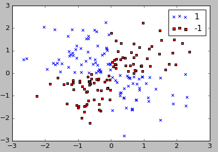
We can clearly see from the xor dataset, we will not be able to separate samples from the positive and negative class very well using a linear hyperplane as the decision boundary from the linear logistic regression or linear SVM model.

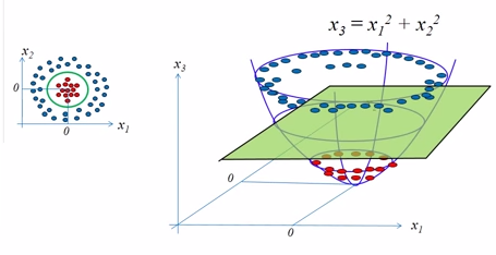
The basic morale of kernel methods is to deal with linearly inseparable data, and to create nonlinear combinations of the original features to project them onto a higher dimensional space via a mapping function $\phi()$ where it becomes linearly separable.

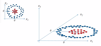
picture source: SVM Tutorial Part2

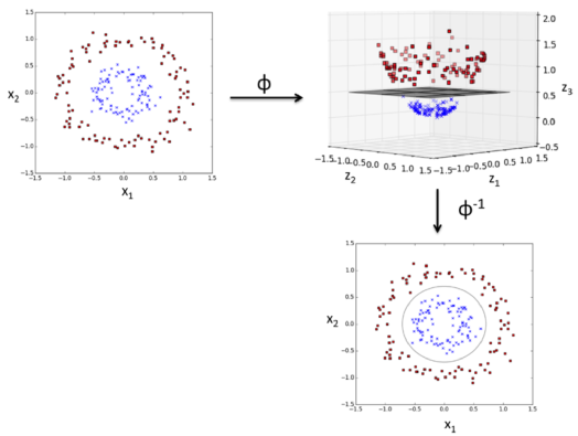
picture source: "Python Machine Learning" by Sebastian Raschka

As shown in the pictures above, we can transform a two-dimensional dataset onto a new three-dimensional feature space where the classes become separable via the following projection:

$$ \phi(x_1, x_2) = (z_1, z_2, z_3) = (x_1, x_2, x_1^2+x_2^2) $$

The mapping allows us to separate the two classes shown in the plot via a linear hyperplane that becomes a nonlinear decision boundary if we project it back ($\phi^{-1}$) onto the original feature space.

To solve a nonlinear problem with SVM:

1. We transform the training data onto a higher dimensional feature space via a mapping function $\phi()$.
2. We train a linear SVM model to classify the data in this new feature space.
3. Then, we can use the same mapping function $\phi()$ to transform unseen data to classify it using the linear SVM model.

However, the problem with this mapping approach is that the constructing the new features is computationally very expensive, especially if we are dealing with high-dimensional data.

This is where the so-called kernel trick comes into play.

The kernel trick avoids the explicit mapping that is needed to get linear learning algorithms to learn a nonlinear function or decision boundary.

To train an SVM, in practice, all we need is to replace the dot product $x^{(i)T} x^{(j)}$ by $\phi \left( x^{(i)} \right ) ^T \phi \left( x^{(j)} \right )$.

In order to avoid the expensive step of calculating this dot product between two points explicitly, we define a so-called kernel function:

$$ k \left( x^{(i)}, x^{(j)} \right) = \phi \left( x^{(i)} \right ) ^T \phi \left( x^{(j)} \right )$$

One of the most widely used kernels is the Radial Basis Function kernel (RBF kernel) or Gaussian kernel, and it is defined like this:

$$ k \left( x^{(i)}, x^{(j)} \right) = exp \left( - \frac {\Vert x^{(i)}-x^{(j)} \Vert^2} {2 \sigma^2} \right ) $$

We usually take simpler form:

$$ k \left(x^{(i)}, x^{(j)}\right) = exp \left( - \gamma {\Vert x^{(i)}-x^{(j)} \Vert^2} \right ) $$

where $\gamma = \frac {1}{2\sigma}$ is a free parameter that need to be optimized.

The term kernel can be thought as a similarity function between a pair of samples.

The minus sign inverts the distance measure into a similarity score.

Due to the exponential term, the resulting similarity score will fall into a range between 1 (for exactly similar samples) and 0 (for very dissimilar samples).

Now that we understand the kernel trick, let's see if we can train a kernel SVM that is able to draw a nonlinear decision boundary that separates the XOR data well or not.

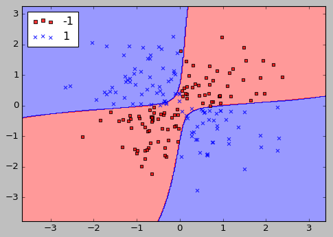
Indeed, the kernel SVM separates the XOR data pretty well.

Here is the code:

import numpy as np

import matplotlib.pyplot as plt
from matplotlib.colors import ListedColormap

def plot_decision_regions(X, y, classifier, test_idx=None, resolution=0.02):
   # setup marker generator and color map
   markers = ('s', 'x', 'o', '^', 'v')
   colors = ('red', 'blue', 'lightgreen', 'gray', 'cyan')
   cmap = ListedColormap(colors[:len(np.unique(y))])

   # plot the decision surface
   x1_min, x1_max = X[:, 0].min() - 1, X[:, 0].max() + 1
   x2_min, x2_max = X[:, 1].min() - 1, X[:, 1].max() + 1
   xx1, xx2 = np.meshgrid(np.arange(x1_min, x1_max, resolution),
   np.arange(x2_min, x2_max, resolution))
   Z = classifier.predict(np.array([xx1.ravel(), xx2.ravel()]).T)
   Z = Z.reshape(xx1.shape)
   plt.contourf(xx1, xx2, Z, alpha=0.4, cmap=cmap)
   plt.xlim(xx1.min(), xx1.max())
   plt.ylim(xx2.min(), xx2.max())

   # plot all samples
   X_test, y_test = X[test_idx, :], y[test_idx]
   for idx, cl in enumerate(np.unique(y)):
      plt.scatter(x=X[y == cl, 0], y=X[y == cl, 1],
               alpha=0.8, c=cmap(idx),
               marker=markers[idx], label=cl)
   # highlight test samples
   if test_idx:
      X_test, y_test = X[test_idx, :], y[test_idx]
      plt.scatter(X_test[:, 0], X_test[:, 1], c='',
               alpha=1.0, linewidth=1, marker='o',
               s=55, label='test set')

# create xor dataset
np.random.seed(0)
X_xor = np.random.randn(200, 2)
y_xor = np.logical_xor(X_xor[:, 0] > 0, X_xor[:, 1] > 0)
y_xor = np.where(y_xor, 1, -1)

# SVM
from sklearn.svm import SVC
svm = SVC(kernel='rbf', random_state=0, gamma=0.10, C=10.0)
svm.fit(X_xor, y_xor)

# draw decision boundary
plot_decision_regions(X_xor, y_xor, classifier=svm)
plt.legend(loc='upper left')
plt.show()

The $\gamma$ parameter, which we set to gamma=0.1, can be understood as a cut-off parameter for the Gaussian sphere.

If we increase the value for $\gamma$, we increase the influence or reach of the training samples, which leads to a softer decision boundary.

In this section, we'll apply RBF kernel SVM to our Iris flower dataset:

import numpy as np

import matplotlib.pyplot as plt
from matplotlib.colors import ListedColormap

def plot_decision_regions(X, y, classifier, test_idx=None, resolution=0.02):
   # setup marker generator and color map
   markers = ('s', 'x', 'o', '^', 'v')
   colors = ('red', 'blue', 'lightgreen', 'gray', 'cyan')
   cmap = ListedColormap(colors[:len(np.unique(y))])

   # plot the decision surface
   x1_min, x1_max = X[:, 0].min() - 1, X[:, 0].max() + 1
   x2_min, x2_max = X[:, 1].min() - 1, X[:, 1].max() + 1
   xx1, xx2 = np.meshgrid(np.arange(x1_min, x1_max, resolution),
   np.arange(x2_min, x2_max, resolution))
   Z = classifier.predict(np.array([xx1.ravel(), xx2.ravel()]).T)
   Z = Z.reshape(xx1.shape)
   plt.contourf(xx1, xx2, Z, alpha=0.4, cmap=cmap)
   plt.xlim(xx1.min(), xx1.max())
   plt.ylim(xx2.min(), xx2.max())

   # plot all samples
   X_test, y_test = X[test_idx, :], y[test_idx]
   for idx, cl in enumerate(np.unique(y)):
      plt.scatter(x=X[y == cl, 0], y=X[y == cl, 1],
               alpha=0.8, c=cmap(idx),
               marker=markers[idx], label=cl)
   # highlight test samples
   if test_idx:
      X_test, y_test = X[test_idx, :], y[test_idx]
      plt.scatter(X_test[:, 0], X_test[:, 1], c='',
               alpha=1.0, linewidth=1, marker='o',
               s=55, label='test set')

from sklearn import datasets
iris = datasets.load_iris()
X = iris.data[:, [2, 3]]
y = iris.target

from sklearn.cross_validation import train_test_split
X_train, X_test, y_train, y_test = train_test_split(X, y, test_size=0.3, random_state=0)

from sklearn.preprocessing import StandardScaler
sc = StandardScaler()
sc.fit(X_train)
X_train_std = sc.transform(X_train)
X_test_std = sc.transform(X_test)

# SVM
from sklearn.svm import SVC
svm = SVC(kernel='rbf', random_state=0, gamma=0.20, C=10.0)
svm.fit(X_train_std, y_train)

X_combined_std = np.vstack((X_train_std, X_test_std))
y_combined = np.hstack((y_train, y_test))

# draw decision boundary
plot_decision_regions(X_combined_std, y_combined,
                      classifier=svm,
                      test_idx=range(105,150))
plt.xlabel('petal length [standardized]')
plt.ylabel('petal width [standardized]')
plt.legend(loc='upper left')
plt.show()

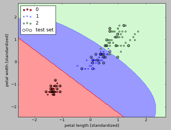
Since we chose a relatively small value for $\gamma$ , the resulting decision boundary of the RBF kernel SVM model will be relatively soft, as shown in the picture above.

If we increase the value of $\gamma$ and observe the effect on the decision boundary:

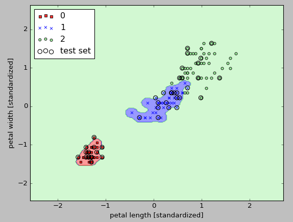
As we can from the picture above, the decision boundary around the classes 0 and 1 is much tighter using a relatively large value of $\gamma$ :

svm = SVC(kernel='rbf', random_state=0, gamma=100.0, C=10.0)

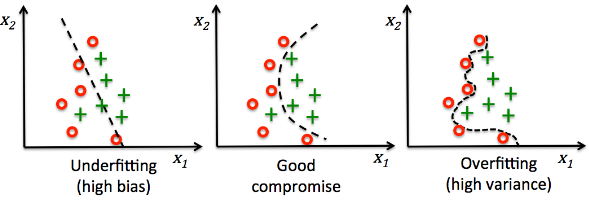
The model fits the training dataset very well, however, such a classifier will likely have a high generalization error for an unseen data.

This demonstrates that the optimization of $\gamma$ also plays an important role in controlling overfitting.

picture source: "Python Machine Learning" by Sebastian Raschka

Machine Learning with scikit-learn

scikit-learn installation

scikit-learn : Features and feature extraction - iris dataset

scikit-learn : Machine Learning Quick Preview

scikit-learn : Data Preprocessing I - Missing / Categorical data

scikit-learn : Data Preprocessing II - Partitioning a dataset / Feature scaling / Feature Selection / Regularization

scikit-learn : Data Preprocessing III - Dimensionality reduction vis Sequential feature selection / Assessing feature importance via random forests

Data Compression via Dimensionality Reduction I - Principal component analysis (PCA)

scikit-learn : Data Compression via Dimensionality Reduction II - Linear Discriminant Analysis (LDA)

scikit-learn : Data Compression via Dimensionality Reduction III - Nonlinear mappings via kernel principal component (KPCA) analysis

scikit-learn : Logistic Regression, Overfitting & regularization

scikit-learn : Supervised Learning & Unsupervised Learning - e.g. Unsupervised PCA dimensionality reduction with iris dataset

scikit-learn : Unsupervised_Learning - KMeans clustering with iris dataset

scikit-learn : Linearly Separable Data - Linear Model & (Gaussian) radial basis function kernel (RBF kernel)

scikit-learn : Decision Tree Learning I - Entropy, Gini, and Information Gain

scikit-learn : Decision Tree Learning II - Constructing the Decision Tree

scikit-learn : Random Decision Forests Classification

scikit-learn : Support Vector Machines (SVM)

scikit-learn : Support Vector Machines (SVM) II

Flask with Embedded Machine Learning I : Serializing with pickle and DB setup

Flask with Embedded Machine Learning II : Basic Flask App

Flask with Embedded Machine Learning III : Embedding Classifier

Flask with Embedded Machine Learning IV : Deploy

Flask with Embedded Machine Learning V : Updating the classifier

scikit-learn : Sample of a spam comment filter using SVM - classifying a good one or a bad one

---

Machine learning algorithms and concepts

Batch gradient descent algorithm

Single Layer Neural Network - Perceptron model on the Iris dataset using Heaviside step activation function

Batch gradient descent versus stochastic gradient descent

Single Layer Neural Network - Adaptive Linear Neuron using linear (identity) activation function with batch gradient descent method

Single Layer Neural Network : Adaptive Linear Neuron using linear (identity) activation function with stochastic gradient descent (SGD)

Logistic Regression

VC (Vapnik-Chervonenkis) Dimension and Shatter

Bias-variance tradeoff

Maximum Likelihood Estimation (MLE)

Neural Networks with backpropagation for XOR using one hidden layer

minHash

tf-idf weight

Natural Language Processing (NLP): Sentiment Analysis I (IMDb & bag-of-words)

Natural Language Processing (NLP): Sentiment Analysis II (tokenization, stemming, and stop words)

Natural Language Processing (NLP): Sentiment Analysis III (training & cross validation)

Natural Language Processing (NLP): Sentiment Analysis IV (out-of-core)

Locality-Sensitive Hashing (LSH) using Cosine Distance (Cosine Similarity)

---

Artificial Neural Networks (ANN)

[Note] Sources are available at Github - Jupyter notebook files

1. Introduction

2. Forward Propagation

3. Gradient Descent

4. Backpropagation of Errors

5. Checking gradient

6. Training via BFGS

7. Overfitting & Regularization

8. Deep Learning I : Image Recognition (Image uploading)

9. Deep Learning II : Image Recognition (Image classification)

10 - Deep Learning III : Deep Learning III : Theano, TensorFlow, and Keras