scikit-learn : Support Vector Machines (SVM)

---

---

Support vector machine (SVM) is a set of supervised learning method, and it's a classifier.

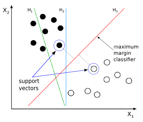
Picture source : Support vector machine

The support vector machine (SVM) is another powerful and widely used learning algorithm.

It can be considered as an extension of the perceptron. Using the perceptron algorithm, we can minimize misclassification errors. However, in SVMs, our optimization objective is to maximize the margin.

As we can see from the picture above, H1 does not separate the classes. H2 does, but only with a small margin. H3 separates them with the maximum margin.

The margin is defined as the distance between the separating hyperplane (decision boundary) and the training samples (support vectors) that are closest to this hyperplane.

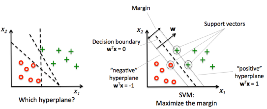
picture source : "Python Machine Learning" by Sebastian Raschka

Once the classifier drawn, it becomes easier to classify a new data instance.

Also, because SVM needs only the support vectors to classify any new data instances, it is quite efficient. In other words, it uses a subset of training points in the decision function ( support vectors), so it is also memory efficient.

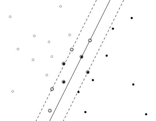
Looks very intuitive, however, the math behind is very complicated. Also, some of the cases cannot be separated by linear approach as shown in the picture below:

Linearly separable:

Non-linearly separable:

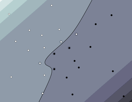
So, there are cases when we need to use non-linear SVM, and it may be quite expensive in terms of calculation.

The bright side of this is SVM is versatile in that different Kernel functions can be specified for the decision function. Common kernels are provided, but it is also possible to specify custom kernels.

1. When there is not too much training data
   1. Training SVMs is computationally heavy
   2. A million instances could be the upper bound of training SVMs
2. When the data has a geometric interpretation
   1. Computer vision problems
3. When we need high precision
4. Note: Parameter tuning needed

Note: this summary is from Machine Learning.

The following picture shows 4 different SVM's classifiers:

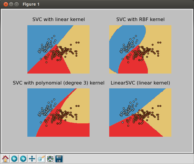
The code that produces the picture looks like this:

import numpy as np
import pylab as pl
from sklearn import svm, datasets

# import some data to play with
iris = datasets.load_iris()
X = iris.data[:, :2]  # we only take the first two features. We could
                      # avoid this ugly slicing by using a two-dim dataset
Y = iris.target

h = .02  # step size in the mesh

# we create an instance of SVM and fit out data. We do not scale our
# data since we want to plot the support vectors
C = 1.0  # SVM regularization parameter
svc = svm.SVC(kernel='linear', C=C).fit(X, Y)
rbf_svc = svm.SVC(kernel='rbf', gamma=0.7, C=C).fit(X, Y)
poly_svc = svm.SVC(kernel='poly', degree=3, C=C).fit(X, Y)
lin_svc = svm.LinearSVC(C=C).fit(X, Y)

# create a mesh to plot in
x_min, x_max = X[:, 0].min() - 1, X[:, 0].max() + 1
y_min, y_max = X[:, 1].min() - 1, X[:, 1].max() + 1
xx, yy = np.meshgrid(np.arange(x_min, x_max, h),
                     np.arange(y_min, y_max, h))

# title for the plots
titles = ['SVC with linear kernel',
          'SVC with RBF kernel',
          'SVC with polynomial (degree 3) kernel',
          'LinearSVC (linear kernel)']


for i, clf in enumerate((svc, rbf_svc, poly_svc, lin_svc)):
    # Plot the decision boundary. For that, we will assign a color to each
    # point in the mesh [x_min, m_max]x[y_min, y_max].
    pl.subplot(2, 2, i + 1)
    Z = clf.predict(np.c_[xx.ravel(), yy.ravel()])

    # Put the result into a color plot
    Z = Z.reshape(xx.shape)
    pl.contourf(xx, yy, Z, cmap=pl.cm.Paired)
    pl.axis('off')

    # Plot also the training points
    pl.scatter(X[:, 0], X[:, 1], c=Y, cmap=pl.cm.Paired)

    pl.title(titles[i])

pl.show()

The code is available from Plot different SVM classifiers in the iris dataset.

In the subsequent section, we'll go over some theoretical backgrounds of SVM and run SVC from sklearn.svm with a selected iris dataset.

The primary reason for having decision boundaries with large margins is that they tend to have a lower generalization error whereas models with small margins are more prone to overfitting (see scikit-learn : Logistic Regression, Overfitting & regularization).

To get the better understanding for the margin maximization, we may want to take a closer look at those positive and negative hyperplanes that are parallel to the decision boundary.

The hyperplanes can be expressed like this:

$$ w_0+w^Tx_{positive}=1$$ $$ w_0+w^Tx_{negative}=-1$$

If we subtract the two linear equations from each other, we get:

$$ w^T \left( x_{positive}-x_{negative} \right) = 2$$

We can normalize this by the length of the vector w, which is defined as follows:

$$ w = \sum_{j=1}^m w_j^2 $$

Then, we'll have the following:

$$ \frac {w^T \left( x_{positive}-x_{negative} \right)} {\Vert w \Vert} = \frac {2} {\Vert w \Vert}$$

The LHS of the equation can then be interpreted as the distance between the positive and negative hyperplane, which is the margin that we want to maximize.

Now the objective function of the SVM becomes the maximization of this margin by maximizing $ \frac {2}{\Vert w \Vert}$ with the constraint of the samples being classified correctly. In other words, all negative samples should fall on one side of the negative hyperplane while all the positive samples should fall behind the positive hyperplane.

So, the constraint should look like this:

$$ w_0+w^Tx^{(i)} = \begin{cases} \ge 1 & \quad if \; y^{(i)}=1 \\ \lt -1 & \quad if \; y^{(i)}=-1 \end{cases}$$

We can write it more compact form:

$$ y^{(i)} \left ( w_0+w^Tx^{(i)} \right ) \ge 1 \quad \forall i $$

We can see we have two choices of implementation, and it depends on a specific SVM:

1. Maximizing $\frac {2} {\Vert w \Vert}$
2. Minimizing $\frac {\Vert w \Vert}{2} $

The reason for introducing the slack variable $\xi$ is that the linear constraints need to be relaxed for nonlinearly separable data to allow convergence of the optimization in the presence of misclassifications under the appropriate cost penalization.

The slack variable simply can be added to the linear constraints:

$$ w^Tx^{(i)} = \begin{cases} \ge 1 & \quad if \; y^{(i)}=1-\xi^{(i)} \\ \lt -1 & \quad if \; y^{(i)}=-1 +\xi^{(i)}\end{cases}$$

So, the new objective to be minimized becomes:

$$ {\Vert w \Vert}^2 + C \left ( \sum_i \xi^{(i)} \right )$$

With the variable C, we can penalize for misclassification.

Large values of C correspond to large error penalties while we are less strict about misclassification errors if we choose smaller values for C.

We can then use the parameter C to control the width of the margin and therefore tune the bias-variance trade-off as shown in the picture below:

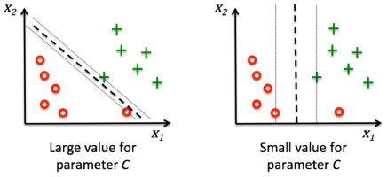
picture source : "Python Machine Learning" by Sebastian Raschka

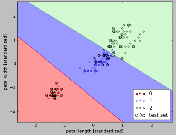
Now that we learned the basic theory for SVM linear kernel, let's train a SVM model to classify our iris dataset:

from sklearn import datasets
import numpy as np
iris = datasets.load_iris()
X = iris.data[:, [2, 3]]
y = iris.target

from sklearn.cross_validation import train_test_split
X_train, X_test, y_train, y_test = train_test_split(X, y, test_size=0.3, random_state=0)

from sklearn.preprocessing import StandardScaler
sc = StandardScaler()
sc.fit(X_train)
X_train_std = sc.transform(X_train)
X_test_std = sc.transform(X_test)

from sklearn.svm import SVC
svm = SVC(kernel='linear', C=1.0, random_state=0)
svm.fit(X_train_std, y_train)

# Decision region drawing
from matplotlib.colors import ListedColormap
import matplotlib.pyplot as plt

def plot_decision_regions(X, y, classifier, test_idx=None, resolution=0.02):
   # setup marker generator and color map
   markers = ('s', 'x', 'o', '^', 'v')
   colors = ('red', 'blue', 'lightgreen', 'gray', 'cyan')
   cmap = ListedColormap(colors[:len(np.unique(y))])

   # plot the decision surface
   x1_min, x1_max = X[:, 0].min() - 1, X[:, 0].max() + 1
   x2_min, x2_max = X[:, 1].min() - 1, X[:, 1].max() + 1
   xx1, xx2 = np.meshgrid(np.arange(x1_min, x1_max, resolution),
   np.arange(x2_min, x2_max, resolution))
   Z = classifier.predict(np.array([xx1.ravel(), xx2.ravel()]).T)
   Z = Z.reshape(xx1.shape)
   plt.contourf(xx1, xx2, Z, alpha=0.4, cmap=cmap)
   plt.xlim(xx1.min(), xx1.max())
   plt.ylim(xx2.min(), xx2.max())

   # plot all samples
   X_test, y_test = X[test_idx, :], y[test_idx]
   for idx, cl in enumerate(np.unique(y)):
      plt.scatter(x=X[y == cl, 0], y=X[y == cl, 1],
               alpha=0.8, c=cmap(idx),
               marker=markers[idx], label=cl)
   # highlight test samples
   if test_idx:
      X_test, y_test = X[test_idx, :], y[test_idx]
      plt.scatter(X_test[:, 0], X_test[:, 1], c='',
               alpha=1.0, linewidth=1, marker='o',
               s=55, label='test set')

X_combined_std = np.vstack((X_train_std, X_test_std))
y_combined = np.hstack((y_train, y_test))

plot_decision_regions(X_combined_std,
                      y_combined, classifier=svm,
                      test_idx=range(105,150))

plt.xlabel('petal length [standardized]')
plt.ylabel('petal width [standardized]')
plt.legend(loc='lower right')
plt.show()

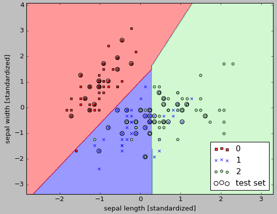
If we use sepal-length and sepal-width instead of petal-length and petal-width:

iris = datasets.load_iris()
# X = iris.data[:, [2, 3]]
X = iris.data[:, [0, 1]]
y = iris.target

The outcome is much worse:

Machine Learning with scikit-learn

scikit-learn installation

scikit-learn : Features and feature extraction - iris dataset

scikit-learn : Machine Learning Quick Preview

scikit-learn : Data Preprocessing I - Missing / Categorical data

scikit-learn : Data Preprocessing II - Partitioning a dataset / Feature scaling / Feature Selection / Regularization

scikit-learn : Data Preprocessing III - Dimensionality reduction vis Sequential feature selection / Assessing feature importance via random forests

Data Compression via Dimensionality Reduction I - Principal component analysis (PCA)

scikit-learn : Data Compression via Dimensionality Reduction II - Linear Discriminant Analysis (LDA)

scikit-learn : Data Compression via Dimensionality Reduction III - Nonlinear mappings via kernel principal component (KPCA) analysis

scikit-learn : Logistic Regression, Overfitting & regularization

scikit-learn : Supervised Learning & Unsupervised Learning - e.g. Unsupervised PCA dimensionality reduction with iris dataset

scikit-learn : Unsupervised_Learning - KMeans clustering with iris dataset

scikit-learn : Linearly Separable Data - Linear Model & (Gaussian) radial basis function kernel (RBF kernel)

scikit-learn : Decision Tree Learning I - Entropy, Gini, and Information Gain

scikit-learn : Decision Tree Learning II - Constructing the Decision Tree

scikit-learn : Random Decision Forests Classification

scikit-learn : Support Vector Machines (SVM)

scikit-learn : Support Vector Machines (SVM) II

Flask with Embedded Machine Learning I : Serializing with pickle and DB setup

Flask with Embedded Machine Learning II : Basic Flask App

Flask with Embedded Machine Learning III : Embedding Classifier

Flask with Embedded Machine Learning IV : Deploy

Flask with Embedded Machine Learning V : Updating the classifier

scikit-learn : Sample of a spam comment filter using SVM - classifying a good one or a bad one

---

Machine learning algorithms and concepts

Batch gradient descent algorithm

Single Layer Neural Network - Perceptron model on the Iris dataset using Heaviside step activation function

Batch gradient descent versus stochastic gradient descent

Single Layer Neural Network - Adaptive Linear Neuron using linear (identity) activation function with batch gradient descent method

Single Layer Neural Network : Adaptive Linear Neuron using linear (identity) activation function with stochastic gradient descent (SGD)

Logistic Regression

VC (Vapnik-Chervonenkis) Dimension and Shatter

Bias-variance tradeoff

Maximum Likelihood Estimation (MLE)

Neural Networks with backpropagation for XOR using one hidden layer

minHash

tf-idf weight

Natural Language Processing (NLP): Sentiment Analysis I (IMDb & bag-of-words)

Natural Language Processing (NLP): Sentiment Analysis II (tokenization, stemming, and stop words)

Natural Language Processing (NLP): Sentiment Analysis III (training & cross validation)

Natural Language Processing (NLP): Sentiment Analysis IV (out-of-core)

Locality-Sensitive Hashing (LSH) using Cosine Distance (Cosine Similarity)

---

Artificial Neural Networks (ANN)

[Note] Sources are available at Github - Jupyter notebook files

1. Introduction

2. Forward Propagation

3. Gradient Descent

4. Backpropagation of Errors

5. Checking gradient

6. Training via BFGS

7. Overfitting & Regularization

8. Deep Learning I : Image Recognition (Image uploading)

9. Deep Learning II : Image Recognition (Image classification)

10 - Deep Learning III : Deep Learning III : Theano, TensorFlow, and Keras