Single Layer Neural Network : Adaptive Linear Neuron using linear (identity) activation function with batch gradient method
In this tutorial, we'll learn another type of single-layer neural network (still this is also a perceptron) called Adaline (Adaptive linear neuron) rule (also known as the Widrow-Hoff rule).
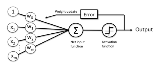
The key difference between the Adaline rule (also known as the Widrow-Hoff rule) and Rosenblatt's perceptron is that the weights are updated based on a linear activation function rather than a unit step function like in the Perceptron model.
Perceptron
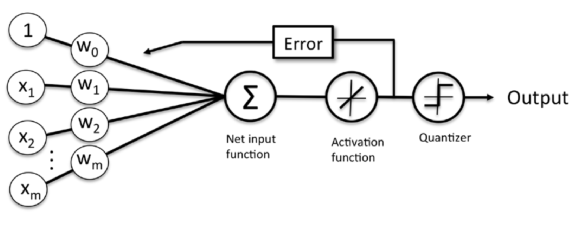
Adaptive linear neuron
The difference is that we're going to use the continuous valued output from the linear activation function to compute the model error and update the weights, rather than the binary class labels.
The perceptron algorithm enables the model automatically learn the optimal weight coefficients that are then multiplied with the input features in order to make the decision of whether a neuron fires or not.
In supervised learning and classification, such an algorithm could then be used to predict if a sample belonged to one class or the other.
In binary classifiers perceptron algorithm, we refer to our two classes as either 1 (positive class) or -1 (negative class).
In the context of neural networks, a perceptron is an artificial neuron using the Heaviside step function as the activation function.
The perceptron algorithm is also termed the single-layer perceptron, to distinguish it from a multilayer perceptron. As a linear classifier, the single-layer perceptron is the simplest feedforward neural network.
We can then define an activation function $\phi(z)$ that takes a linear combination of certain input values $x$ and a corresponding weight vector $w$ , where $z$ is the so-called net input ($z = w_1x_1 + ... + w_mx_m$).
$$w=\begin{bmatrix} w_1 \\ . \\ . \\ . \\ w_m \\ \end{bmatrix}, x=\begin{bmatrix} x_1 \\ . \\ . \\ . \\ x_m \\ \end{bmatrix} $$For our case (binary), we can have:
$$\text if \quad \sum_{i=1}w_ix_i > \theta \quad \text then \quad \phi = 1 $$ $$\text else \quad \sum_{i=1}w_ix_i < \theta \quad \text then \quad \phi = -1 $$If we set $x_0=1$ and $w_0=-\theta$, we can have more compact form:
$$\text if \quad \sum_{i=0}w_ix_i > 0 \quad \text then \quad \phi(z) = 1 $$ $$\text else \quad \sum_{i=0}w_ix_i < 0 \quad \text then \quad \phi(z) = -1 $$ where $$z=\sum_{i=0}w_ix_i$$Or more compact form.
- Heaviside step activation function: $$\phi(z) = \begin{cases}1 & z > 0 \\ -1 & \text{otherwise} \end{cases}$$
- Linear activation function: $$\phi(z) = z$$
Update of each weight $w_j$ in the weight vector $w$ can be written as:
$$w_j : = w_j + \Delta w_j$$The value of $\Delta w_j$ , which is used to update the weight $w_j$, is calculated as the following:
- Heaviside step activation function: $$\Delta w_j=\eta(y^{(i)}-\hat y^{(i)})x_j^{(i)}$$
- Linear activation function: $$\Delta w_j=-\eta \frac{\partial J}{\partial w_j}$$ where $\eta$ is learning rate ($0.0 < \eta <1.0$), $y^{(i)}$ is the true class label of the i-th training sample, and $\hat y^{(i)}$ is the predicted class label.
One of the most critical tasks in supervised machine learning algorithms is to minimize cost function.
In the case of Adaptive linear neuron, we can define the cost function J to learn the weights as the Sum of Squared Errors (SSE) between the calculated outcome and the true class label:
$$J(w)=\frac{1}{2}\sum_{i}(y^{(i)}-\phi(z^{(i)}))^2$$
COmpared with the unit step function, the advantages of this continuous linear activation function are:
- This cost function is differentiable. So, the partial derivative of the SSE cost function with respect to the jth weight is:
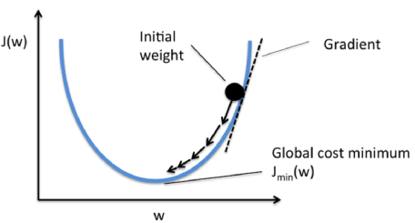
- Because it is convex, we can use a simple and powerful, optimization algorithm called gradient descent to find the weights that minimize our cost function to classify the samples in the Iris dataset.
$$\frac{\partial J}{\partial w_j}=-\sum_{i}(y^{(i)}-\phi(z^{(i)}))x_{j}^{(i)}$$
where $i$ is the sample # and $j$ is the feature # (dimension of a dataset).
Although the adaptive linear learning rule looks identical to the perceptron rule, the $\phi(z^{(i)})$ with $z^{(i)}=w^Tx^{(i)}$ is a real number and not an integer class label.
Also, the weight update is calculated based on all samples in the training set (instead of updating the weights incrementally after each sample), which is why this approach is also referred to as batch gradient descent.
We can minimize a cost function by taking a step into the opposite direction of a gradient that is calculated from the whole training set, and this is why this approach is also called as batch gradient descent.
Since the perceptron rule and Adaptive Linear Neuron are very similar, we can take the perceptron implementation that we defined earlier and change the fit method so that the weights are updated by minimizing the cost function via gradient descent.
Here is the source code:
import numpy as np

class AdaptiveLinearNeuron(object):
   def __init__(self, rate = 0.01, niter = 10):
      self.rate = rate
      self.niter = niter

   def fit(self, X, y):
      """Fit training data
      X : Training vectors, X.shape : [#samples, #features]
      y : Target values, y.shape : [#samples]
      """

      # weights
      self.weight = np.zeros(1 + X.shape[1])

      # Number of misclassifications
      self.errors = []

      # Cost function
      self.cost = []

      for i in range(self.niter):
         output = self.net_input(X)
         errors = y - output
         self.weight[1:] += self.rate * X.T.dot(errors)
         self.weight[0] += self.rate * errors.sum()
         cost = (errors**2).sum() / 2.0
         self.cost.append(cost)
      return self

   def net_input(self, X):
      """Calculate net input"""
      return np.dot(X, self.weight[1:]) + self.weight[0]

   def activation(self, X):
      """Compute linear activation"""
      return self.net_input(X)

   def predict(self, X):
      """Return class label after unit step"""
      return np.where(self.activation(X) >= 0.0, 1, -1)


import matplotlib.pyplot as plt
import numpy as np
import pandas as pd

df = pd.read_csv('https://archive.ics.uci.edu/ml/machine-learning-databases/iris/iris.data', header=None)

y = df.iloc[0:100, 4].values
y = np.where(y == 'Iris-setosa', -1, 1)
X = df.iloc[0:100, [0, 2]].values

fig, ax = plt.subplots(nrows=1, ncols=2, figsize=(8, 4))

# learning rate = 0.01
aln1 = AdaptiveLinearNeuron(0.01, 10).fit(X,y)

ax[0].plot(range(1, len(aln1.cost) + 1), np.log10(aln1.cost), marker='o')
ax[0].set_xlabel('Epochs')
ax[0].set_ylabel('log(Sum-squared-error)')
ax[0].set_title('Adaptive Linear Neuron - Learning rate 0.01')

# learning rate = 0.01
aln2 = AdaptiveLinearNeuron(0.0001, 10).fit(X,y)

ax[1].plot(range(1, len(aln2.cost) + 1), aln2.cost, marker='o')
ax[1].set_xlabel('Epochs')
ax[1].set_ylabel('Sum-squared-error')
ax[1].set_title('Adaptive Linear Neuron - Learning rate 0.0001')
plt.show()
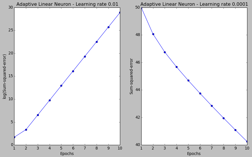
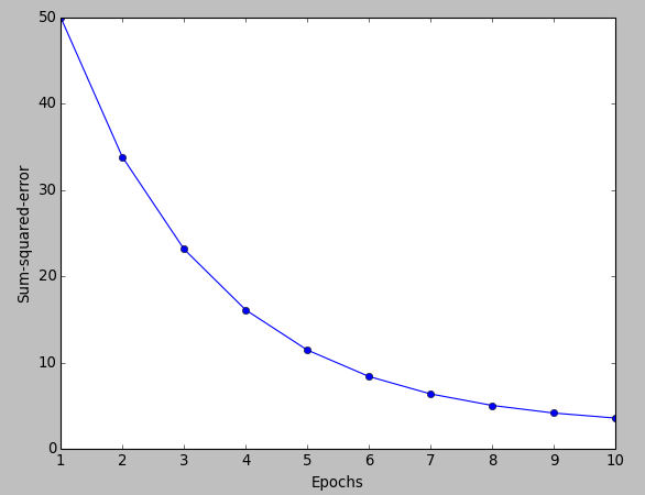
As we can see in the resulting cost function plots below, we have two different types of issues.
The left one shows what could happen if we choose a learning rate that is too large. Instead of minimizing the cost function, the error becomes larger in every epoch because we overshoot the global minimum.
On the other hand, we can see that the cost decreases for the plot on the right side. That's because we chose the learning rate $\eta=0.0001$ is so small that the algorithm would require a very large number of epochs to converge.
The following figure demonstrates how we change the value of a particular weight parameter to minimize the cost function $J$ (left). The figure on the right illustrates what happens if we choose a learning rate that is too large, we overshoot the global minimum:
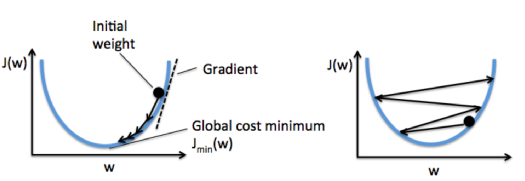
Picture from "Python Machine Learning by Sebastian Raschka, 2015"
Feature scaling is a method used to standardize the range of independent variables or features of data. In data processing, it is also known as data normalization and is generally performed during the data preprocessing step.
Gradient descent is one of the many algorithms that benefit from feature scaling.
Here, we will use a feature scaling method called standardization, which gives our data the property of a standard normal distribution.In machine learning, we can handle various types of data, e.g. audio signals and pixel values for image data, and this data can include multiple dimensions.
Feature standardization makes the values of each feature in the data have zero-mean (when subtracting the mean in the enumerator) and unit-variance.
This method is widely used for normalization in many machine learning algorithms (e.g., support vector machines, logistic regression, and neural networks).
This is typically done by calculating standard scores.
The general method of calculation is to determine the distribution mean and standard deviation for each feature. Next we subtract the mean from each feature. Then we divide the values (mean is already subtracted) of each feature by its standard deviation.
- from Feature scaling
So, to standardize the $j$-th feature, we just need to subtract the sample mean $\mu_j$ from every training sample and divide it by its standard deviation $sigma_j$:
$$ x_j^\prime=\frac {x_j-\mu_j}{\sigma_j}$$where $x_j$ is a vector consisting of the $j$-th feature values of all training samples $n$.
We can standardize by using the NumPy methods mean and std:
X_std = np.copy(X)
X_std[:,0] = (X[:,0] - X[:,0].mean()) / X[:,0].std()
X_std[:,1] = (X[:,1] - X[:,1].mean()) / X[:,1].std()
After the standardization, we will train the Linear model again using the not so small learning rate of $\eta = 0.01$:
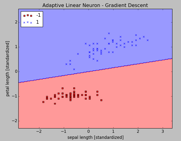
Here is our new code for the two pictures above:
import matplotlib.pyplot as plt
import numpy as np
import pandas as pd
from matplotlib.colors import ListedColormap

class AdaptiveLinearNeuron(object):
   def __init__(self, rate = 0.01, niter = 10):
      self.rate = rate
      self.niter = niter

   def fit(self, X, y):
      """Fit training data
      X : Training vectors, X.shape : [#samples, #features]
      y : Target values, y.shape : [#samples]
      """

      # weights
      self.weight = np.zeros(1 + X.shape[1])

      # Number of misclassifications
      self.errors = []

      # Cost function
      self.cost = []

      for i in range(self.niter):
         output = self.net_input(X)
         errors = y - output
         self.weight[1:] += self.rate * X.T.dot(errors)
         self.weight[0] += self.rate * errors.sum()
         cost = (errors**2).sum() / 2.0
         self.cost.append(cost)
      return self

   def net_input(self, X):
      """Calculate net input"""
      return np.dot(X, self.weight[1:]) + self.weight[0]

   def activation(self, X):
      """Compute linear activation"""
      return self.net_input(X)

   def predict(self, X):
      """Return class label after unit step"""
      return np.where(self.activation(X) >= 0.0, 1, -1)

def plot_decision_regions(X, y, classifier, resolution=0.02):
   # setup marker generator and color map
   markers = ('s', 'x', 'o', '^', 'v')
   colors = ('red', 'blue', 'lightgreen', 'gray', 'cyan')
   cmap = ListedColormap(colors[:len(np.unique(y))])

   # plot the decision surface
   x1_min, x1_max = X[:,  0].min() - 1, X[:, 0].max() + 1
   x2_min, x2_max = X[:, 1].min() - 1, X[:, 1].max() + 1
   xx1, xx2 = np.meshgrid(np.arange(x1_min, x1_max, resolution),
   np.arange(x2_min, x2_max, resolution))
   Z = classifier.predict(np.array([xx1.ravel(), xx2.ravel()]).T)
   Z = Z.reshape(xx1.shape)
   plt.contourf(xx1, xx2, Z, alpha=0.4, cmap=cmap)
   plt.xlim(xx1.min(), xx1.max())
   plt.ylim(xx2.min(), xx2.max())

   # plot class samples
   for idx, cl in enumerate(np.unique(y)):
      plt.scatter(x=X[y == cl, 0], y=X[y == cl, 1],
      alpha=0.8, c=cmap(idx),
      marker=markers[idx], label=cl)

df = pd.read_csv('https://archive.ics.uci.edu/ml/machine-learning-databases/iris/iris.data', header=None)

y = df.iloc[0:100, 4].values
y = np.where(y == 'Iris-setosa', -1, 1)
X = df.iloc[0:100, [0, 2]].values

# standardize
X_std = np.copy(X)
X_std[:,0] = (X[:,0] - X[:,0].mean()) / X[:,0].std()
X_std[:,1] = (X[:,1] - X[:,1].mean()) / X[:,1].std()

# learning rate = 0.01
aln = AdaptiveLinearNeuron(0.01, 10)
aln.fit(X_std,y)

# decision region plot
plot_decision_regions(X_std, y, classifier=aln)

plt.title('Adaptive Linear Neuron - Gradient Descent')
plt.xlabel('sepal length [standardized]')
plt.ylabel('petal length [standardized]')
plt.legend(loc='upper left')
plt.show()

plt.plot(range(1, len(aln.cost) + 1), aln.cost, marker='o')
plt.xlabel('Epochs')
plt.ylabel('Sum-squared-error')
plt.show()
Machine Learning with scikit-learn
scikit-learn installation
scikit-learn : Features and feature extraction - iris dataset
scikit-learn : Machine Learning Quick Preview
scikit-learn : Data Preprocessing I - Missing / Categorical data
scikit-learn : Data Preprocessing II - Partitioning a dataset / Feature scaling / Feature Selection / Regularization
scikit-learn : Data Preprocessing III - Dimensionality reduction vis Sequential feature selection / Assessing feature importance via random forests
Data Compression via Dimensionality Reduction I - Principal component analysis (PCA)
scikit-learn : Data Compression via Dimensionality Reduction II - Linear Discriminant Analysis (LDA)
scikit-learn : Data Compression via Dimensionality Reduction III - Nonlinear mappings via kernel principal component (KPCA) analysis
scikit-learn : Logistic Regression, Overfitting & regularization
scikit-learn : Supervised Learning & Unsupervised Learning - e.g. Unsupervised PCA dimensionality reduction with iris dataset
scikit-learn : Unsupervised_Learning - KMeans clustering with iris dataset
scikit-learn : Linearly Separable Data - Linear Model & (Gaussian) radial basis function kernel (RBF kernel)
scikit-learn : Decision Tree Learning I - Entropy, Gini, and Information Gain
scikit-learn : Decision Tree Learning II - Constructing the Decision Tree
scikit-learn : Random Decision Forests Classification
scikit-learn : Support Vector Machines (SVM)
scikit-learn : Support Vector Machines (SVM) II
Flask with Embedded Machine Learning I : Serializing with pickle and DB setup
Flask with Embedded Machine Learning II : Basic Flask App
Flask with Embedded Machine Learning III : Embedding Classifier
Flask with Embedded Machine Learning IV : Deploy
Flask with Embedded Machine Learning V : Updating the classifier
scikit-learn : Sample of a spam comment filter using SVM - classifying a good one or a bad one
Machine learning algorithms and concepts
Batch gradient descent algorithmSingle Layer Neural Network - Perceptron model on the Iris dataset using Heaviside step activation function
Batch gradient descent versus stochastic gradient descent
Single Layer Neural Network - Adaptive Linear Neuron using linear (identity) activation function with batch gradient descent method
Single Layer Neural Network : Adaptive Linear Neuron using linear (identity) activation function with stochastic gradient descent (SGD)
Logistic Regression
VC (Vapnik-Chervonenkis) Dimension and Shatter
Bias-variance tradeoff
Maximum Likelihood Estimation (MLE)
Neural Networks with backpropagation for XOR using one hidden layer
minHash
tf-idf weight
Natural Language Processing (NLP): Sentiment Analysis I (IMDb & bag-of-words)
Natural Language Processing (NLP): Sentiment Analysis II (tokenization, stemming, and stop words)
Natural Language Processing (NLP): Sentiment Analysis III (training & cross validation)
Natural Language Processing (NLP): Sentiment Analysis IV (out-of-core)
Locality-Sensitive Hashing (LSH) using Cosine Distance (Cosine Similarity)
Artificial Neural Networks (ANN)
[Note] Sources are available at Github - Jupyter notebook files1. Introduction
2. Forward Propagation
3. Gradient Descent
4. Backpropagation of Errors
5. Checking gradient
6. Training via BFGS
7. Overfitting & Regularization
8. Deep Learning I : Image Recognition (Image uploading)
9. Deep Learning II : Image Recognition (Image classification)
10 - Deep Learning III : Deep Learning III : Theano, TensorFlow, and Keras
Ph.D. / Golden Gate Ave, San Francisco / Seoul National Univ / Carnegie Mellon / UC Berkeley / DevOps / Deep Learning / Visualization