scikit-learn : Data Preprocessing II - (Partitioning a dataset / Feature scaling / Feature Selection / Regularization)

bogotobogo.com site search:

Partitioning training and test sets

We will prepare a new dataset, the Wine dataset which is available from the UCI machine learning repository ( https://archive.ics.uci.edu/ml/datasets/Wine ).

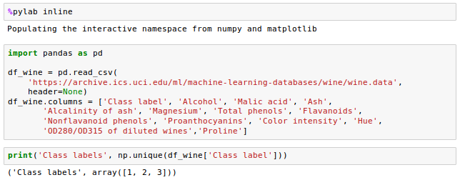
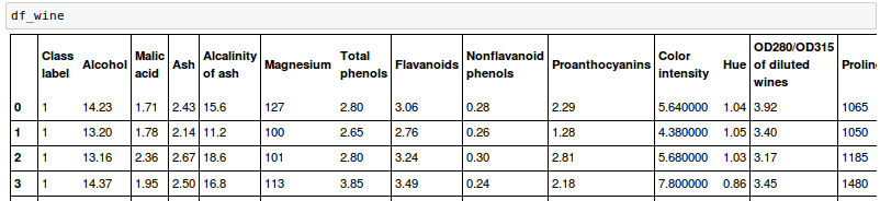
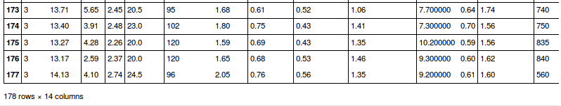
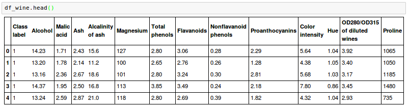
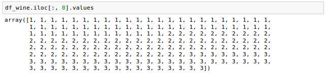
It has 178 wine samples with 13 features for different chemical properties:

The samples belong to one of three different classes, 1, 2, and 3, which refer to the three different types of grapes that have been grown in different regions in Italy.

In order to randomly partition this dataset into a separate test and training dataset, we'll use the train_test_split() from scikit-learn's cross_validation submodule:

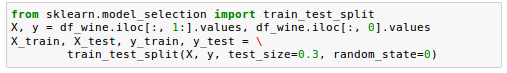
As we can see from the code above, we assigned the feature columns 1-13 to the variable $X$, and we assigned the class labels (the 1st column) to the variable $y$.

After that, we used the train_test_split() method to randomly split $X$ and $y$ into separate training and test datasets.

We set the test_size=0.3, which means that we assigned 30 percent of the wine samples to X_test and y_test, and the remaining 70 percent of the samples were assigned to X_train and y_train, respectively:

Feature scaling

Feature scaling is a method used to standardize the range of features. It is also known as data normalization (or standardization) and is a crucial step in data preprocessing.

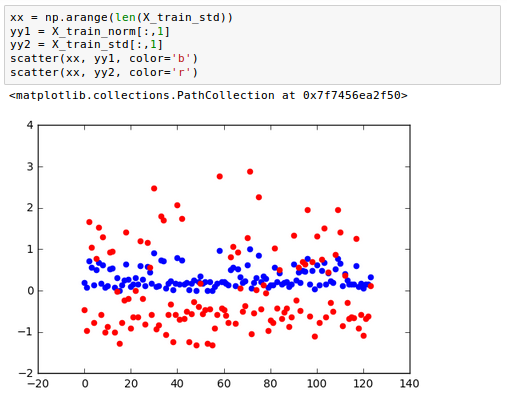
Suppose we have two features where one feature is measured on a scale from 0 to 1 and the second feature is 1 to 100 scale.

When we compute the squared error function or a Euclidean distance for the k-nearest neighbors (KNN), our algorithm will mostly be busy in handling the larger errors in the second feature.

Usually, normalization refers to the re-scaling the features in the range of [0, 1].

To normalize our data, we can apply the min-max scaling to each feature column, where the new value $x_{norm}$ of a sample $x$ can be computed as below:

$$x_{norm} = \frac {x-x_{min}}{x_{max}-x_{min}}$$

Let's see how it's done in scikit-learn:

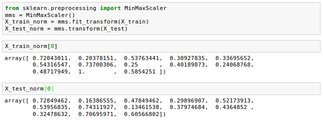
Though normalization via min-max scaling is useful to keep values in a bounded interval, standardization can be more practical when we want the feature columns to have a normal distribution. This makes the algorithm less sensitive to the outliers in contrast to min-max scaling:

$$x_{std} = \frac {x-\mu}{\sigma}$$

where $\mu$ is the sample mean of a particular feature column and $\sigma$ the corresponding standard deviation, respectively.

The following table demonstrate the difference between the two feature scaling, standardization and normalization on a sample dataset from 0 to 5:

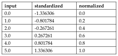
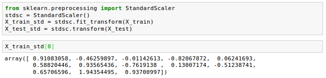
Let's see how the standardization scikit-learn is implemented:

Here is the comparison of the two - standardization and normalization:

Note that we fit the StandardScaler only once on the training data. Then, we use those parameters we got from the training to transform the test set or any new data point.

Feature selection

Whenever we see that a model performs much better on a training dataset than on the test dataset, we should doubt that there might be an overfitting or high variance in our model.

In other words, our model fits the parameters too closely to the training data but has greater generalization (or prediction) errors for real data.

Here are some ways of reducing the generalization error:

Choose a simpler model with fewer parameters.
Introduce a penalty for complexity via regularization.
Reduce the dimensionality of the data.
Collect more training data. This may not be applicable.

Regularization

Regularization is a way of tuning or selecting the preferred level of model complexity so that our model performs better at predicting.

If we skip this regularization step, our model may not be generalized well to real data while the model fits well to the training dataset.

The regularization introduced a penalty for large individual weights so that we can reduce the complexity of a model.

We can have two types of norms of the regularization: L1 and L2:

$$ L1_{norm} : \sum_i \vert w_i \vert$$ $$ L2_{norm} : \sum_i \Vert w_i \Vert^2$$

Unlike L2 regularization, L1 regularization yields sparse feature vectors since most feature weights will be zero.

The sparsity, in practice, can be very useful when we have a high-dimension dataset that has many irrelevant features (more irrelevant dimensions than samples).

If that's the case, the L1 regularization can be used as a way of feature selection.

L1 regularization & sparsity of a solution

We want to make balances between the data (unpenalized cost function) term and regularization (penalty or bias) term.

$$ J(\mathbf w) = \color{green}{ \frac{1}{2}(\mathbf y-\mathbf w \mathbf x^T)(\mathbf y-\mathbf w \mathbf x^T)^T } + \color{red}{ \lambda \mathbf w \mathbf w^T } \tag 1$$

Solution can be like this:

$$ \mathbf w = \mathbf y \mathbf x(\mathbf x^T \mathbf x+\lambda \mathbf I)^{-1} \tag 2 $$

Via the regularization parameter $\lambda$, we can then control how well we fit the training data while keeping the weights small.

Our primary goal is to find the combination of weight coefficients that minimize the cost function for the training data.

As we can see from Eq. 1, we added regularization term which is a penalty term to the cost function to encourage smaller weights. By adding the term, we penalize large weights!

By increasing the value of $\lambda$, we increase the regularization strength, which shrinks the weights towards zero and decrease the dependence of our model on the training data.

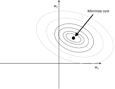
For L2 regularization, we can think of the process similar to the diagram below where The shaded circle represents L2 term:

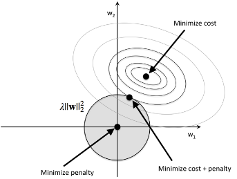
Here, our weight coefficients cannot exceed our regularization budget($C$):

$$ \mathbf w \mathbf w^T \le C $$

In other words, the combination of the weight coefficients cannot fall outside the shaded area while we still want to minimize the cost function($J$).

Under the penalty constraint, our best effort is to choose the point where the L2 ball intersects with the contours of the unpenalized cost function. The larger the value of the regularization parameter $\lambda$ gets, the faster the penalized cost function grows, which leads to a narrower L2 ball.

For example, if we increase the regularization parameter towards infinity, the weight coefficients will become effectively zero, denoted by the center of the L2 ball.

Now, let's tale about L1 regularization.

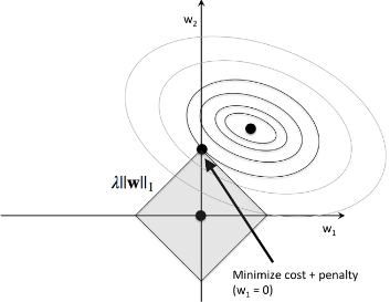
picture source : Python Machine Learning by Sebastian Raschka

In the picture, the diamond shape represents the budget for L1 regularization term. As we can see the contour of the cost function touches the L1 diamond at $w_1 = 0$. Since the contours of an L1 regularized system are sharp, it is more likely that the optimum (intersection between the ellipses of the cost function and the boundary of the L1 diamond) is located on the axes, which encourages sparsity.

In L2 case, the center of the ellipse (the minimum cost) should falls on the axis when budget circle of L2 intersects the ellipses of the cost function. So, in L2, sparsity rarely occurs.

L1 regularization in scikit-learn

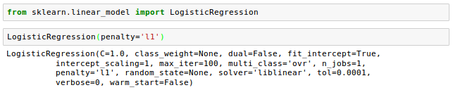
Let's see how scikit-learn supports L1 regularization:

We get the the following sparse solution when the L1 regularized logistic regression is ppplied to the standardized Wine data:

The accuracies for training and test are both 98 percent, which suggests no overfitting in our model.

When we access the intercept terms via the intercept_ attribute, it returns an array with three values:

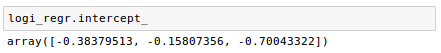
Because we the fit the LogisticRegression object on a multiclass dataset, by default, it uses the One-vs-Rest (OvR).

How can we get the weight vector for each class?

We can use coef_ attribute as shown in the code below:

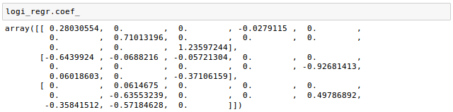
The weight array returned from coef_ attribute contains three rows of weight coefficients, one weight vector for each class.

The array has quite a few zero entries, which means the weight vectors are sparse. As we discussed earlier, L1 regularization can be used a way of doing feature selection, and indeed we just trained a model that is few irrelevant features in this dataset.

Each row consists of 13 weights where each weight is multiplied by the respective feature in the 13-dimensional Wine dataset to compute the net input:

$$ z = \sum_{j=0}^m x_jw_j = \mathbf w^T \mathbf x $$

Behavior of L1 regularization

How the behavior of L1 regularization looks like?

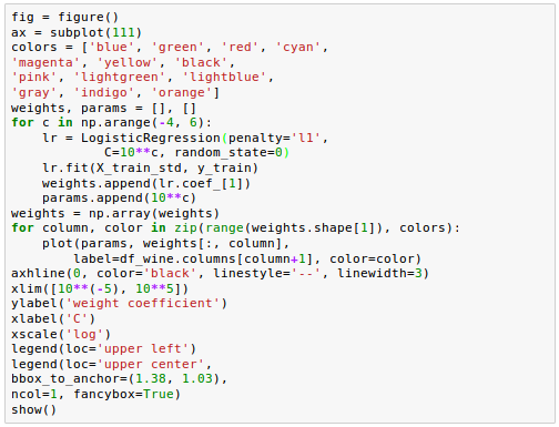
Let's plot the weight coefficients of the different features for different regularization strengths:

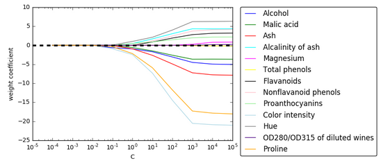
As we can see from the picture, all features weights will be zero if we penalize the model with a strong regularization parameter ($ C = \frac {1}{\lambda} \lt 0.1 $).

Github repository

Source is available from bogotobogo-Machine-Learning .

Next:

Data Preprocessing III - Dimensionality reduction vis Sequential feature selection / Assessing feature importance via random forests